DataCleaner example code

from obspy.core.stream import read
from obspy.core.inventory import read_inventory
from tiskitpy import DataCleaner, SpectralDensity

# Read data and inventory
stream = read('data/XS.S11D.LH.2016.12.11.mseed', 'MSEED')
inv = read_inventory('data/XS.S11_decimated.station.xml', 'STATIONXML')

# Calculate a Datacleaner that will subtract `*1`, then `*2`, then `*H`
dc = DataCleaner(stream, ['*1','*2','*H'])

[INFO] z_threshold=3, rejected 4% of windows (3/84)
[INFO] z_threshold=3, rejected 4% of windows (3/84)
[INFO] z_threshold=3, rejected 4% of windows (3/84)
[INFO] z_threshold=3, rejected 4% of windows (3/84)

# Clean the data, then construct a stream with original and cleaned channels
stream_cleaned = dc.apply(stream)
z_compare = stream.select(channel='*Z') + stream_cleaned.select(channel='*Z')

[INFO] Correcting traces in the frequency domain

# If you print and plot the stream "normally", they have the same channel names
print(z_compare)
z_compare.plot()

2 Trace(s) in Stream:
XS.S11D..LHZ | 2016-12-10T23:59:59.992583Z - 2016-12-11T23:59:59.992583Z | 1.0 Hz, 86401 samples
XS.S11D..LHZ | 2016-12-10T23:59:59.992583Z - 2016-12-11T23:59:59.992583Z | 1.0 Hz, 86401 samples

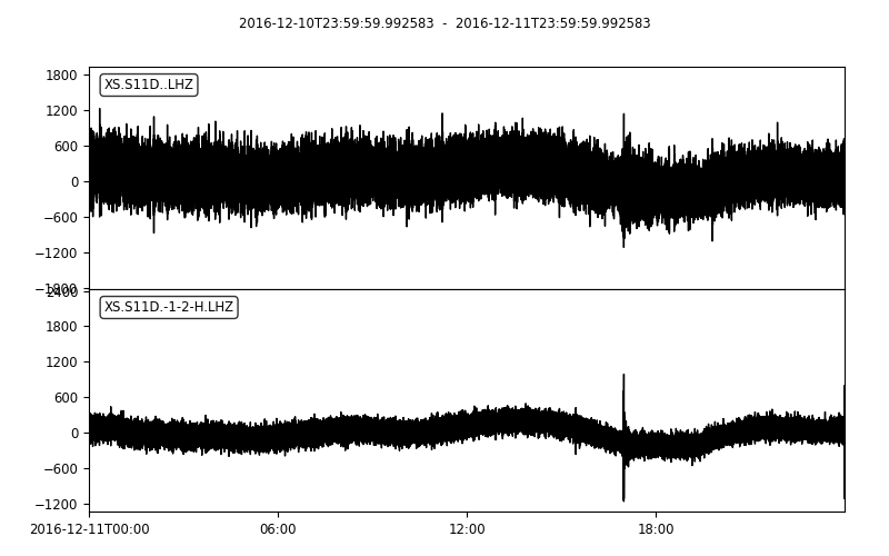
# If you convert the Stream to its CleanedStream subclass, the tiskit_py ids are printed and plotted
z_compare = CleanedStream(z_compare)
print(z_compare)
z_compare.plot(outfile='3_DataCleaner_tagged_timeseries_cleanedstream.png')

2 Trace(s) in Stream:
XS.S11D..LHZ       | 2016-12-10T23:59:59.992583Z - 2016-12-11T23:59:59.992583Z | 1.0 Hz, 86401 samples
XS.S11D.-1-2-H.LHZ | 2016-12-10T23:59:59.992583Z - 2016-12-11T23:59:59.992583Z | 1.0 Hz, 86401 samples

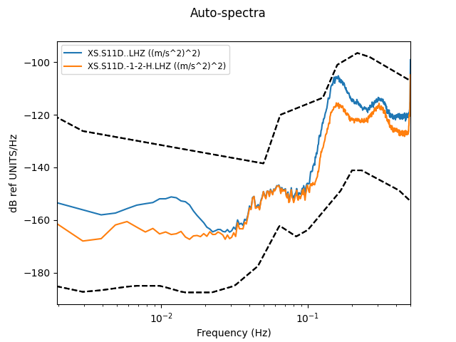
# compare spectral densities
# (tiskitpy plot() automatically includes CleanSequence information)
sd_compare = SpectralDensity.from_stream(z_compare, inv=inv)
sd_compare.plot(overlay=True)

[INFO] z_threshold=3, rejected 5% of windows (4/84)