Compliance Calculation example code

"""
Calculate compliance for a half-space model, and compare it to
the theoretical value and the one calculated from derived data
"""
from obspy import UTCDateTime
from obspy.core.stream import Trace
import numpy as np
import matplotlib.pyplot as plt

from tiskitpy import (SpectralDensity, SeafloorSynthetic, ResponseFunctions,
                      Compliance)

# PARAMETERS
rho, vp, vs = 2500, 4000, 2000  # kg/m^3, m/s, m/s
no_noise = True

# Almost perfectly leveled Z to get measureable compliance without cleaning
kwargs = {'Z_offset_angles': (0.01, 0),
          'earth_model': [[1000, rho, vp, vs],
                          [1000, rho, vp, vs],
                          [1000, rho, vp, vs]]}
if no_noise is True:
    kwargs['Z_offset_angles'] = (0.00, 0)
    kwargs['noise_pressure'] = ([[0.001, -150], [1, -150]], True)
    kwargs['noise_seismo'] =   ([[0.001, -250], [1, -250]], True)

# Create noise model
noise_model = SeafloorSynthetic(**kwargs)

# Create synthetic data from the noise model
n_days = 10
s_rate = 1
sta_code = 'SYNTH'
synth_start_time = '2024-01-01T00'
resp_trace = Trace(np.ones(86400*n_days*s_rate),
                   header={'sampling_rate': s_rate,
                           'starttime': UTCDateTime(synth_start_time),
                           'channel': 'LHZ'})

# Specify sensitivities that keep the compliance values in the passband
s_sensitivity = 1e13  # Below 1e10 and above 1e15, compliance is too low
p_sensitivity = 1e5  # Below 1e2 and above 1e7, compliance is too high

data_synth, sources, inv_synth = noise_model.streams(
    resp_trace, s_response=s_sensitivity, p_response=p_sensitivity,
    station=sta_code, forceInt32=True)

# If I use the standard prol4pi (or kaiser4pi or dpss4) taper, high frequency
# values are too high (because pressure drops faster than motion?)
sd_synth = SpectralDensity.from_stream(data_synth, inv=inv_synth, windowtype='dpss1')

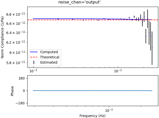
# Theoretical compliance assuming c << vp, vs
ncompl_theoretical = - vp**2 / (2 * rho * vs**2 * (vp**2 - vs**2))

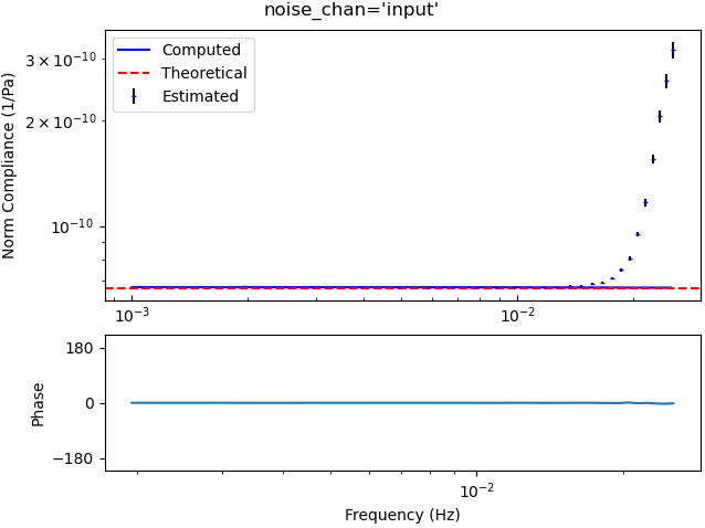
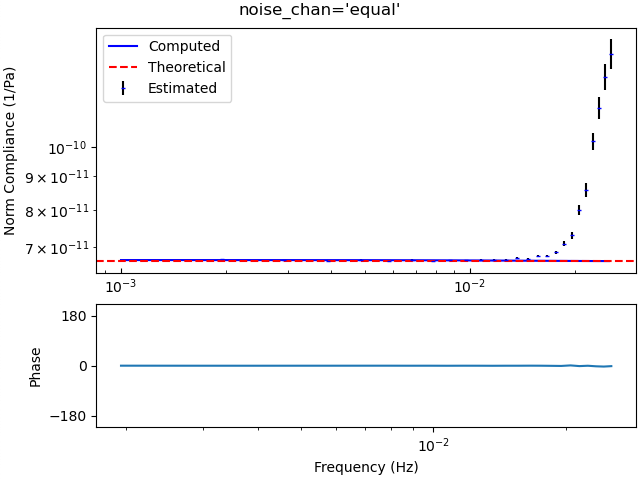
# Compare theoretical, calculated and "measured" compliance for different
# assumptions of which channel the noise is on
for noise_chan in ("output", "input", "equal", "unknown"):
    # Calculate normalized compliance from the data
    rfs = ResponseFunctions(sd_synth,  '*LDG', ['*LHZ'],
                            noise_channel=noise_chan)
    ncompl_est = Compliance.from_response_functions(rfs, noise_model.water_depth)
    # Calculate normalized compliance directly from the model
    ncompl_computed = Compliance.from_seafloor_synthetic(noise_model)

    # Plot comparison of theoretical, model-computed and "data-estimated" compliances
    axa, axp = ncompl_est.plot(show=False)
    axa.plot(ncompl_computed.freqs, np.abs(ncompl_computed.values), c='b', label='Computed')
    axa.axhline(np.abs(ncompl_theoretical), ls='--', c='r', label='Theoretical')
    axa.legend()
    plt.suptitle(f'{noise_chan=}')
    plt.show()
    plt.close()