SeafloorSynthetic example code

"""
Create synthetic OBS training data

- Read in real data from a quiet continental site
- Create a noise model using the SeafloorSynthetic class with default values
- Add the two together
- Save the result
- Also save:
    - The original input data
    - The calculated compliance

"""
from pathlib import Path

import numpy as np
from obspy import read, read_inventory, UTCDateTime
import matplotlib.pyplot as plt

from tiskitpy import SpectralDensity, SeafloorSynthetic, PSDVals

data_file = 'data/G.TAM_2010059-2010069.mseed'  # post-Maule eq
inv_file = 'data/G.TAM.2010.station.xml'
wdepth = 2400
station = 'SYNV1'
wt = 'prol4pi'  # hamming and prol1pi don't have enough broadband noise rejection

# Read the real data and its metadata
real_data = read(data_file, 'MSEED')
resp_trace = real_data[0].copy()

# Change the start time to "hide" its provenance
resp_trace.stats.start_time = UTCDateTime(2024,1,1)
inv = read_inventory(inv_file, 'STATIONXML')
# Extract the instrument response
s_response=inv.select(channel='LHZ')[0][0][0].response

# Create the noise model and synthetic data stream
noise_tilt_max = PSDVals.sloped_freqs_and_values(-180, -30, -3, 0.1, .25)
noise_model = SeafloorSynthetic(noise_tilt_max=noise_tilt_max,
                              noise_tilt_variance=30)

# PLOT noise model using SeafloorSynthetic's intrinsic method
noise_model.plot(outfile='noise_model.png')

# Create the synthetic and sources data streams
data_synth, sources, inv_synth = noise_model.streams(
    real_data[0], s_response=s_response, p_response = 100.,
    station=station)
noisePSDs = noise_model.PSDs

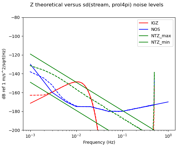
# Compare the PSDs of the noise sources' waveforms to their theoretical valus
sd_sources = SpectralDensity.from_stream(sources, windowtype=wt)
fig, ax = plt.subplots()
for component, color in zip(('IGZ', 'NOS', 'NTZ_max', 'NTZ_min'), ('r', 'b', 'g', 'g')):
    ax.semilogx(noisePSDs[component].freqs, noisePSDs[component].values, color, label=component)
    ax.semilogx(sd_sources.freqs, 10*np.log10(sd_sources.autospect('*' + component[:3])), color+'--')
ax.set_ylim(-200, -80)
ax.set_xlabel('Frequency (Hz)')
ax.set_ylabel('dB ref 1 m/s^2/sqrt(Hz)')
plt.suptitle(f'Z theoretical versus sd(stream, {wt}) noise levels')
plt.legend()
plt.show()

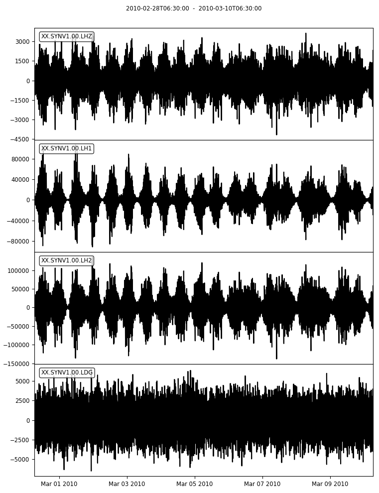
# PLOT synthetic time series
data_synth.plot(equal_scale=False)

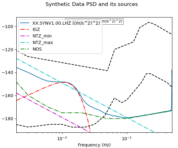
# PLOT synthetic PSD versus SeafloorSynthetic components
sd_synth = SpectralDensity.from_stream(data_synth, inv=inv_synth, windowtype=wt)
ax = sd_synth.plot_one_autospectra(f'XX.{station}.00.LHZ')
ylim = ax.get_ylim()
for label, color in zip(('IGZ', 'NTZ_min', 'NTZ_max', 'NOS'), ('r', 'm', 'c', 'g')):
    ax.plot(noisePSDs[label].freqs, noisePSDs[label].values,
            color=color, label=label, linestyle='-.')
ax.set_ylim(ylim)
ax.legend()
plt.gcf().suptitle('Synthetic Data PSD and its sources')
plt.show()

# Add the real and synthetic data together
data = data_synth.copy()
data.select(channel='LHZ')[0].data += real_data.select(channel='LHZ')[0].data
data.select(channel='LH1')[0].data += real_data.select(channel='LHN')[0].data
data.select(channel='LH2')[0].data += real_data.select(channel='LHE')[0].data

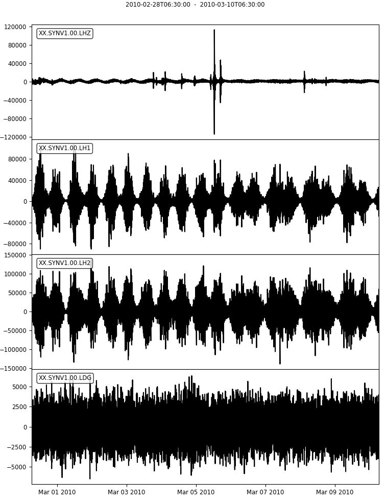
# PLOT synthetic + real time series
data.plot(equal_scale=False)

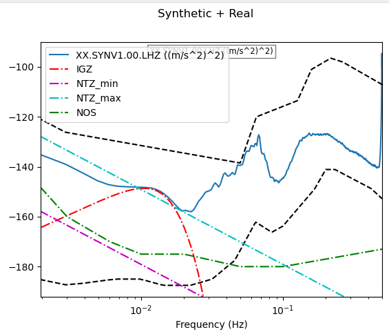
# PLOT synthetic + real PSD versus SeafloorSynthetic components
sd_synth = SpectralDensity.from_stream(data, inv=inv_synth, windowtype=wt)
ax = sd_synth.plot_one_autospectra(f'XX.{station}.00.LHZ')
ylim = ax.get_ylim()
for label, color in zip(('IGZ', 'NTZ_min', 'NTZ_max', 'NOS'), ('r', 'm', 'c', 'g')):
    ax.plot(noisePSDs[label].freqs, noisePSDs[label].values,
            color=color, label=label, linestyle='-.')
ax.set_ylim(ylim)
ax.legend()
plt.gcf().suptitle('Synthetic + Real')
plt.show()

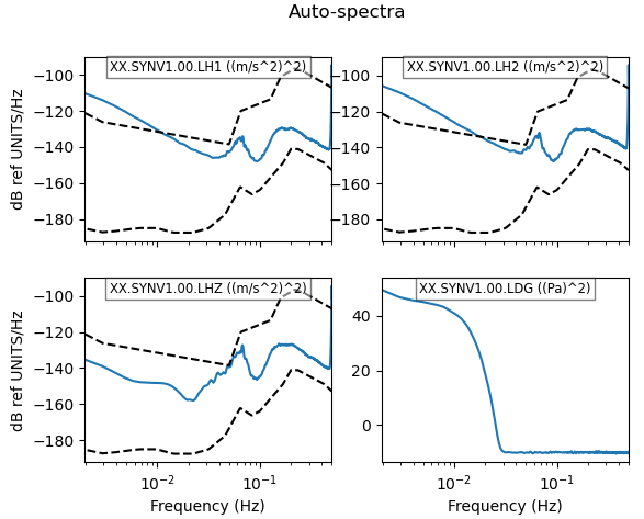
sd_data = SpectralDensity.from_stream(data, windowtype=wt)
# PLOT synthetic+real PSD
sd_data.plot()

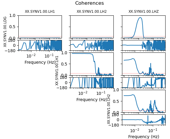
# PLOT synthetic+real coherence
sd_data.plot_coherences()