PeriodicTransient example code

First, read some data and create a PeriodicTransient objet

from tiskitpy.rptransient import PeriodicTransient
from obspy.core.stream import read

# Transient parameters
transient_starttime = '2009-01-23T09:00:00'
transient_clips = (-1000, 1000)
transient_period = 3600
dp = 1

stream = read('data/LSVSB.Z.sample.mseed', 'MSEED')
trace_train = stream.select(channel="*MHZ")[0].copy()

# PERIODIC TRANSIENT
pt = PeriodicTransient("hourly_glitch",
                       transient_period,
                       dp=dp, clips=transient_clips,
                       transient_starttime=transient_starttime)

The Transient parameters are simply guesses, although we know that the period is about one hour

Next, run calc_timing()

print('\n\n***RUNNING CALC_TIMING***')
pt.calc_timing(trace_train)

The program starts by plotting stacked waveforms, spaced by transient_period and with clip levels given by transient clips

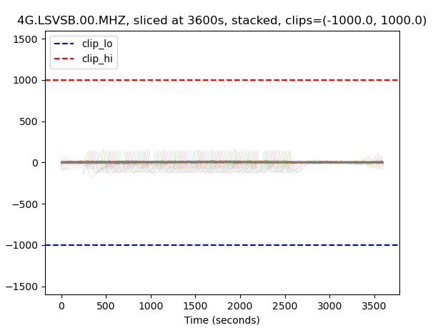
It writes out the clip levels and asks the user to enter new ones. Here, the user entered -200, 200:

Enter clip levels containing all transients (RETURN for current value) (-1000.0, 1000.0): -200, 200

The result is better, but still a bit too much:

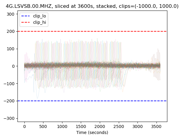
The user now enters -150, 150:

Enter clip levels containing all transients (RETURN for current value) (-1000.0, 1000.0): -150, 150

The result is pretty good now:

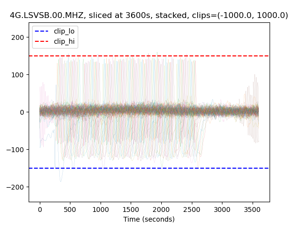
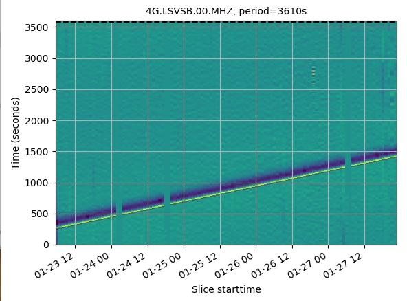
The user now hits the return key, which accepts the current values and moves on to estimating the periodic transient period:

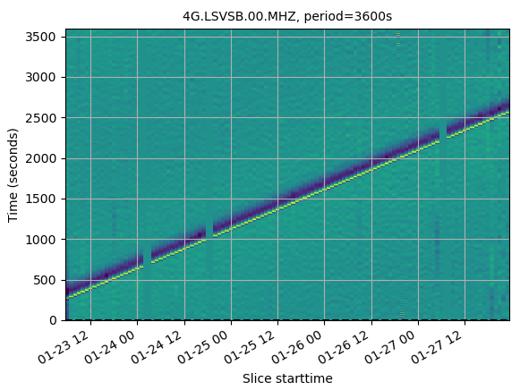
The slope is positive, so the user enters a larger value: 3610

If the slope is positive, INCREASE the period
Enter new test period  (RETURN uses current value) [3600]: 3610

The slope is still positive, so the user enters a larger value:

Enter new test period  (RETURN uses current value) [3610]: 3620

The slope is pretty flat, maybe a little bit positive, so the user enters a slightly larger value:

Enter new test period  (RETURN uses current value) [3620]: 3621

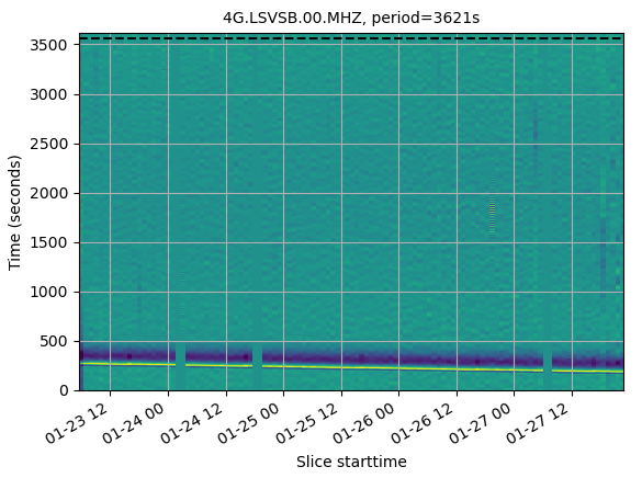
The slope is now negative, go back to the previous value, then accept it by hitting return at the next question

Enter new test period  (RETURN uses current value) [3621]: 3620
Enter new test period  (RETURN uses current value) [3621]:

The code moves on to the transient_starttime:

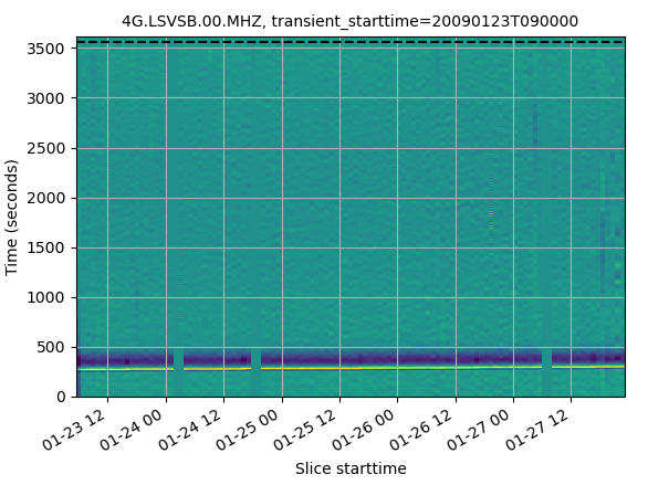
The dashed line is a little to far “below” the start of the transient (actually, it’s above, but as the vertical axis wraps, one can consider it to be a few hundred seconds below)

If the dotted line is beneath the transient, enter a POSTIVE offset
transient_starttime = 2009-01-23T09:00:00.000000Z
Enter offset seconds  (RETURN uses current value) [0]: 200

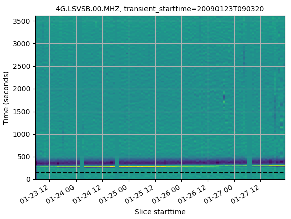
The result is better, the dashed line is below the transients, but not too far. Accept the latest time by hitting return

One could now put the found parameters at the top of the file:

# Transient parameters
transient_starttime = '2009-01-23T09:03:200'
transient_clips = (-150, 150)
transient_period = 3620
dp = 1

(the dp value controls how far to either side of the transient period that calc_transient() will consider when trying to find the “exact” period)

Next, run calc_transient()

Using the newfound transient value (which are also stored in the pt object), we can run calc_transient():

pt.calc_transient(trace_train, plots=True)

The first plot shows which traces were selected, which ones were rejected because of a known earthquake, and which ones were rejected because their variance was anomalously:

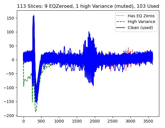
You have to close it manually, after which the code calculates the “dirac comb” it will multipy each transient by, testing periods from transient_starttime - dp to ``transient_starttime + dp` for the best overlap of transients. Once it has finished, it shows the “ideal” dirac comb, plus the one it will use to calculate the transient (which lacks “teeth” around known earthquakes and high variance windows)

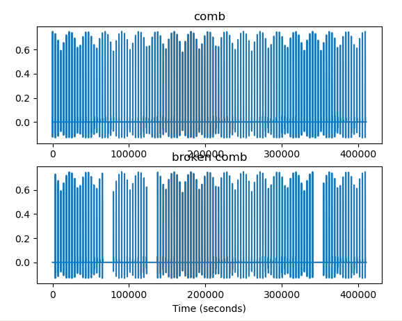
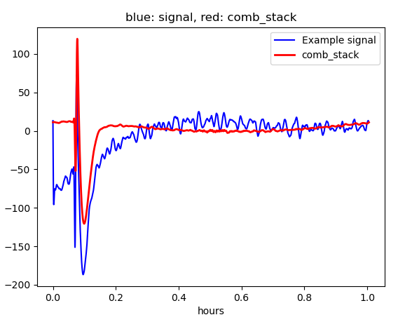
When you close this window, the code averages all aligned transients (using the “broken comb” and plots the result, next to a sample data window)

Running comb_calc("hourly_glitch": 3620.00s+-1.0, clips=(-150, 150), training and matching freq bounds=(True, 0.05), transient_starttime=2009-01-23T09:03:20.000000Z
    Rejecting high-variance slices (>2.295e+06+3*4.763e+05)...1 of 113 rejected
    Running comb_stack(period=3619.0s)
    Running _comb_remove_all
    Running comb_stack(period=3620.0s)
    Running _comb_remove_all
    Running comb_stack(period=3621.0s)
    Running _comb_remove_all
    best period found=3620.13
    Running comb_stack(period=3620.1276643498136s)

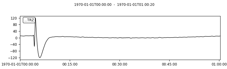
Finally, the code plots the best-fit transient, by itself

Lastly, run remove_transient()

stream_before = stream.copy()  # This is simply for comparison later
trace = stream.select(channel="*MHZ")[0]
trace_after = pt.remove_transient(trace, plots=True)

The program plots the original data, the cleaned data (channel code=”CLN”) and the synthetic transient that was removed from the data (channel code=’SYN’)

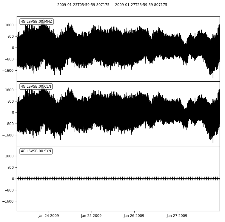
We don’t see any difference! That is because the data are dominated by microseisms which are much stronger that the infragravity waves and therefore not strongly affected by the glitch. calc_timing() and calc_transients() filter out, by default, the microseisms (parameters freq_HP and freq_LP )

If we want to see the effect of our work, we need to filter in a similar fashion.

First, we import the corrected trace into stream:

# Replace the Z component trace with the one with the removed transient
for i, t in enumerate(stream):
    if t.stats.channel == 'MHZ':
        print('replacing channel')
        stream[i] = trace_after
        break

Then we put the before and after traces in a stream, change the before stream’s location code to 99 (so that we can tell which is which in the plot), lowpass filter the data at the same frequency as calc_timing and calc_transient.

# Compare filtered stream before and after
trace_before = stream_before.select(channel='MHZ').copy()
trace_after = stream.select(channel='MHZ').copy()
trace_before[0].stats.location='99'
stream_compare = trace_before + trace_after
stream_compare.filter("lowpass", freq=pt.freq_LP)
stream_compare.plot()

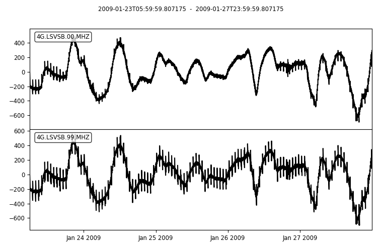
The new waveform lacks most of the hourly transients that plagued the original data. But there are still a few sections with the transients. Room for improvement…